Visualization and exploration of high-dimensional data is a ubiquitous challenge across disciplines. Widely used techniques such as principal component analysis (PCA) aim to identify dominant trends in one dataset. However, in many settings we have datasets collected under different conditions, e.g., a treatment and a control experiment, and we are interested in visualizing and exploring patterns that are specific to one dataset. This paper proposes a method, contrastive principal component analysis (cPCA), which identifies low-dimensional structures that are enriched in a dataset relative to comparison data. In a wide variety of experiments, we demonstrate that cPCA with a background dataset enables us to visualize dataset-specific patterns missed by PCA and other standard methods. We further provide a geometric interpretation of cPCA and strong mathematical guarantees. An implementation of cPCA is publicly available, and can be used for exploratory data analysis in many applications where PCA is currently used.
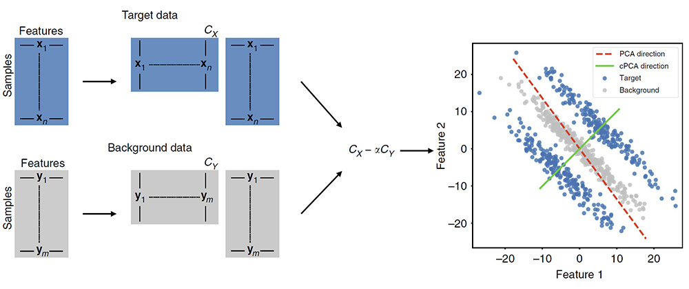
Schematic Overview of cPCA. To perform cPCA, compute the covariance matrices C X , C Y of the target and background datasets. The singular vectors of the weighted difference of the covariance matrices, C X − α · C Y , are the directions returned by cPCA. As shown in the scatter plot on the right, PCA (on the target data) identifies the direction that has the highest variance in the target data, while cPCA identifies the direction that has a higher variance in the target data as compared to the background data. Projecting the target data onto the latter direction gives patterns unique to the target data and often reveals structure that is missed by PCA. Specifically, in this example, reducing the dimensionality of the target data by cPCA would reveal two distinct clusters
The Mexican example caught my attention:
Relationship between ancestral groups in Mexico
In previous examples, we have seen that cPCA allows the user to discover subclasses within a target dataset that are not labeled a priori. However, even when subclasses are known ahead of time, dimensionality reduction can be a useful way to visualize the relationship within groups. For example, PCA is often used to visualize the relationship between ethnic populations based on genetic variants, because projecting the genetic variants onto two dimensions often produces maps that offer striking visualizations of geographic and historic trends26,27. But again, PCA is limited to identifying the most dominant structure; when this represents universal or uninteresting variation, cPCA can be more effective at visualizing trends.
The dataset that we use for this example consists of single nucleotide polymorphisms (SNPs) from the genomes of individuals from five states in Mexico, collected in a previous study28. Mexican ancestry is challenging to analyze using PCA since the PCs usually do not reflect geographic origin within Mexico; instead, they reflect the proportion of European/Native American heritage of each Mexican individual, which dominates and obscures differences due to geographic origin within Mexico (see Fig. 4a). To overcome this problem, population geneticists manually prune SNPs, removing those known to derive from Europeans ancestry, before applying PCA. However, this procedure is of limited applicability since it requires knowing the origin of the SNPs and that the source of background variation to be very different from the variation of interest, which are often not the case.
Relationship between Mexican ancestry groups. a PCA applied to genetic data from individuals from 5 Mexican states does not reveal any visually discernible patterns in the embedded data. b cPCA applied to the same dataset reveals patterns in the data: individuals from the same state are clustered closer together in the cPCA embedding. c Furthermore, the distribution of the points reveals relationships between the groups that matches the geographic location of the different states: for example, individuals from geographically adjacent states are adjacent in the embedding. c Adapted from a map of Mexico that is originally the work of User:Allstrak at Wikipedia, published under a CC-BY-SA license, sourced from https://commons.wikimedia.org/wiki/File:Mexico_Map.svg
As an alternative, we use cPCA with a background dataset that consists of individuals from Mexico and from Europe. This background is dominated by Native American/European variation, allowing us to isolate the intra-Mexican variation in the target dataset. The results of applying cPCA are shown in Fig. 4b. We find that individuals from the same state in Mexico are embedded closer together. Furthermore, the two groups that are the most divergent are the Sonorans and the Mayans from Yucatan, which are also the most geographically distant within Mexico, while Mexicans from the other three states are close to each other, both geographically as well as in the embedding captured by cPCA (see Fig. 4c). See also Supplementary Fig. 6 for more details.
So, by using a background dataset, it discovers patterns in a single target dataset via dimensionality reduction, that standard dimensionality reduction techniques do not discover. Maybe useful for some prehistoric populations, too…