The recently published preprint Assessing the Performance of qpAdm, by Harney, Patterson, Reich, & Wakeley at bioRxiv (2020) offers some interesting clues about what previous papers using qpAdm might have done right, and – more importantly – what they might have done wrong.
Since it doesn’t make much sense to repeat what this open access paper says within quotes, I will try to use short sentences or rework them to sum it up, illustrating best practices and common pitfalls with what I believe are corresponding examples with Steppe-related populations to date, with an emphasis on Bell Beakers. Most of the text below is therefore either copied or reworked from the paper.
I. Estimating ancestry with qpAdm
1. Standard model
The chief purpose of qpAdm is to identify a subset of plausible models of a population’s ancestry from a larger set of possible models. p-values (less than 5%) and admixture proportions outside of the relevant range (0,1) should be used to reject implausible models.
The distribution of p-values is not expected to be uniform, but rather show an appreciable change of being above the 5% cutoff – hence incorrect models should fall largely below p=0.05%.
While the distribution of p-values differs between optimal and non-optimal models, for individual replicates the most optimal model is not necessarily assigned the highest p-value. In the ideal models simulated in the paper, it corresponded to 48% of cases. Therefore, the authors caution against p-value ranking.
One might think that this should be common knowledge by now, but if you are used to reading about qpAdm analyses, you know that chasing after greater p-values is the norm rather than the exception. Not only geneticists, but also researchers from many different fields constantly misunderstand what it means (and what it doesn’t), being probably among the most common type of formal errors in published results and discussions.
2. Accuracy of admixture proportion estimates
qpAdm accurately estimates admixture proportions, even when applied to data of lower coverage and quality. However, the increase in variance and potential bias is additive:
- Pseudohaploidy.
- Ancient damage, even when unevenly distributed, is unlikely to cause a user to identify a non-optimal model as plausible. However, when target and source populations have different rates of damage, the optimal model is almost always deemed impossible (in general, avoid designs combining ancient and modern populations).
- Special care needed for lower sample size (in particular N=1 and large amounts of missing data) in target or source populations, because it reduces power to reject non-optimal models. Especially when the optimal source population is relatively undifferentiated from all other populations considered.
NOTE. Some of the qpAdm models for Bell Beakers below use a single sample (or few samples) as target and/or source populations, but there doesn’t seem to be damage or large amounts of missing data.
3. Comparing admixture models
The traditional strategy of using a base set of reference populations to compare multiple targets and sources has several drawbacks, among them the missing of optimal source populations and the creation of non-equivalent (and thus not comparable) models.
Best practice recommendation is to create a set of “rotating” models, where a single set of populations is selected for analyses, and all other populations serve as reference.
- It is not overly stringent when optimal data are not available, because it identifies related models as possible (say, Yamnaya as a source for Corded Ware when the optimal Steppe-related source population is not available).
- More importantly, the addition of the optimal source populations as reference enables qpAdm to differentiate between models that would otherwise be indistinguishable, by rejecting non-optimal models.
This strategy has been recently applied to Steppe-related populations by contrasting Corded Ware (Srubnaya) against Afanasievo as references for the Tocharian-related Shirenzigou samples in Ning et al. (2019), an analysis recently confirmed with more coeval samples in Wang et al. (2020). I have also applied a similar strategy for Steppe-related populations in previous posts: see examples for Bell Beakers & Mycenaeans, “Steppe ancestry” populations, Italic peoples & Etruscans, Proto-Corded Ware Late Trypillian, or Chemurchek & Shirenzigou.
3.1. Ascertainment bias
Ascertainment bias is not necessarily an issue, since the optimal model is identified as plausible in at least 90% of cases. I was really surprised by this, though, because this has been one of the main warnings about relying on ancient DNA in most publications, and I have complained about it myself. Time to let go of this suspicion then.
Furthermore, in a comment at Gene Expression relative to the use of shotgun sequenced samples, Harney states that:
My guess would be that the results of qpAdm will be affected if some of the populations are captured and some are shotgun sequenced, as populations that exhibit similar patterns of missing data may appear more or less similar than they actually are. So I would advise that users exercise similar caution when using these different types of data.
As you can see, my models of Bell Beakers from Yamnaya_Kalmykia.SG were overfitted for northern groups compared to the results below for all Yamnaya source populations. This might have been due to the mix of shotgun samples (from Yamnaya Kalmykia and Germany Corded Ware), but my personal guess is that, much like I cautioned about at the end of that post, the usual culprit of such ‘great’ p-values seems to be the number and nature of outgroups (see below 4.1. Number of reference populations).
3.2. Missing data
It is usually better to use the “allsnps: YES” option to improve the ability of qpAdm to distinguish between plausible and non-optimal models, especially when the rate of missing data is elevated: possibly already when >25%, certainly when >80%.
3.3. Unadmixed populations
It is important to consider first one- or two-way models, because models in which only a single source population contributed ancestry to the target population can often be successfully modeled as the product of two-way admixture between the true source and another one, with models being typically rejected based on contributions greater than 100% (“infeasible”) rather than on p-values. In other words, always look for the subsets and, if the fits improve, test them, too.
I would say that another closely related problem is trying to find the optimal source among closely related ones when the admixture proportion is small. The case of Italy Bell Beakers below is illustrative of how the good fits obtained have (probably) more to do with a majority of South-Eastern EEF-related ancestry derived from a source close to Hungary Baden samples, and not with the Steppe-related source. A similar warning should be considered for other good fits for CWC, probably based mostly on Central-Northern EEF-like (i.e. GAC-related) ancestry.
4. Challenging admixture scenarios
4.1. Number of reference populations
A large number of reference populations is useful to distinguish between optimal and non-optimal admixture models and reducing standard errors of admixture proportion estimates, but it tends to make computed p-values unreliable.
The exact maximum number depends on population history and total amount of data in the analysis, but – theoretically – plausible models start to get rejected from 30 reference populations.
In my models of Bell Beakers, I didn’t want to increase the number of references, trying to imitate as closely as possible the strategy of Wang et al. (2018, 2019) & Ning et al. (2019). By replacing Villabruna (i.e. the WHG reference) I probably selected to remove one of the worst possible outgroups, particularly useful for contrasting ancestry among ‘northern’ European Beakers (i.e. those more likely to show CWC admixture). Seeing now that the number of empirically acceptable samples can be up to 30, it’s evident that adding references instead of replacing them is the ideal strategy.
NOTE. Indeed, results below for Yamnaya_Kalmykia are not comparable to those I posted months ago, because samples merged from Wang et al. (2018) came from an amateur pipeline, not like this one from the Reich Lab curated dataset, and the comparison doesn’t even involve the same sources (and in some cases, the targets). So, this is mostly my impression based on some unlikely good fits found then for “northern” Beakers, and the bad fits found now even for East BBC groups, but I won’t lose time testing that. You are welcome to do it, though.
It seems difficult to understand how the ‘O9’ reference set in Lazaridis (2016) had become, as many other things, a sort of empirical tradition against which only a detailed simulation-based paper like this could fight. This prevalent empiricism based on copying the previous, rather scarce experience with poorly understood tools seems a little unsciency in hindsight, and reveals our desire to tread carefully out of fear of misunderstanding the consequences of poor choices more than a conscious selection of a conservative model.
4.2. Continuous gene flow
The underlying assumption of qpAdm is that admixture occurs in a single pulse over a small interval of time. Continuous gene flow over a prolonged period of time results in ancestry from multiple sources, which makes estimates of admixture proportions not meaningful, especially when:
1) The duration of exchange of ancestry is much longer than what is supposed in qpAdm. As far as we know, “Steppe ancestry” might have been exchanged for more than a millennium within the opened Middle to Late Eneolithic CHG-related mating network of the north Pontic area between steppe- and forest-steppe-related hunter-gatherers, and later between the (partially Khvalynsk-derived) Sredni Stog population and the Steppe Maykop-like ancestry proper of Proto-Corded Ware.
2) All Bell Beaker populations likely formed in the same splitting event from Yamnaya Hungary, so a comparison between them (or derived populations), especially when admixing with similar Steppe-related (Corded Ware) and EEF-related populations – such as Central European ones – is bound to show results consistent with them being the result of an admixture between ancestral populations common to all groups assessed; nothing more, nothing less. For more on this, see my formal comparison of Lower Rhine vs. East BBC.
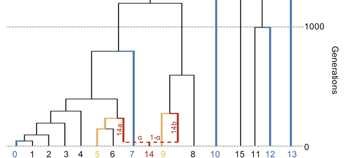
3) By symmetry, each Bell Beaker population might be as much the source of other Bell Beakers as any of the latter might be the source of the former. Plotted in the PCA, these populations appear to form clines between each other, and alternative demographic models are possible for each cluster. To simplify the conundrum, you can assess an expansion of “Steppe ancestry” among Beakers by naïvely selecting Steppe-rich Beakers and combining them with EEF populations (to prove, say, a Dutch Beaker origin of all Bell Beakers), as much as you can assess an expansion of “EEF ancestry” by selecting EEF-rich Beakers and combining them with Steppe populations (to prove, say, an Iberian Beaker origin of all Bell Beakers). None of these models is likely at all from any point of view, be it genetic, archaeological, or linguistic.
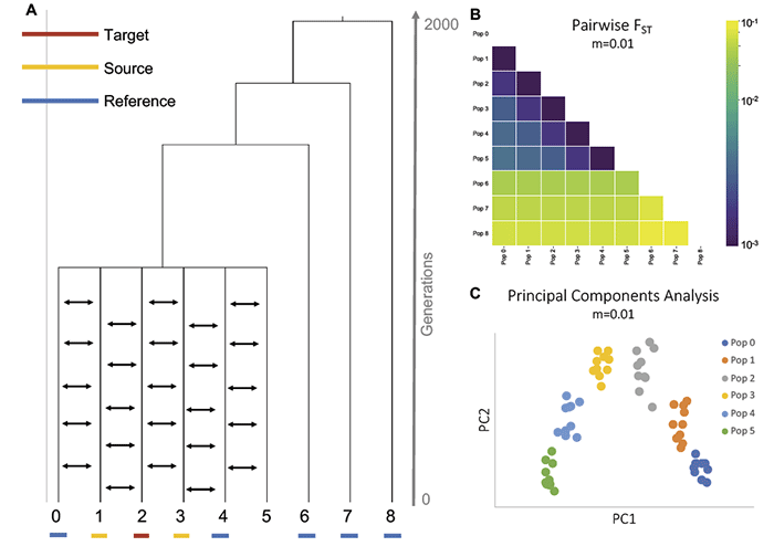
With a high admixture rate (m=0.01 compared to m=0.001 and m=0.0001) it is even more difficult to distinguish between population histories that involve continuous migration from those involving pulses of admixture.
NOTE. If you plan on understanding the pitfalls of future papers assessing the origin of “Steppe ancestry” among different populations, especially among Corded Ware and among Bell Beakers, I suggest you read carefully this section of the paper and try to brand this image of continuous gene flow on your brain. It will pop up every step of the “Steppe-related” way ahead.
4.3. Formally distinguish source from target
Supposedly, using other f-statistics “it might be possible” to determine the relationship of the populations, but the referenced Lipson (2020) merely offers interesting ideas for likely improvement in the selection of admixture events rather than carefully simulated models, as Harney et al. (2020) do.
For the time being, the use of these suggestions seems to open another door to more uncertainty and thus for confusing experiments of ancestry magic at a time when certainty is what matters.
In words of Harney et al. (2020), that in my opinion should accompany every formal or informal report of qpAdm:
there is nothing to prevent a naïve user from attempting to model this relationship as the product of admixture using qpAdm.
Needless to say, it’s not really a personal attribute – “user” – but rather impersonal – “use”: Naïve uses of qpAdm are found everywhere, and have been done by everyone as far as I can remember, including the experienced authors of this paper. Bad uses and misinterpretations are not going to stop any time soon, so a focus on the person instead of the specific setting is a wrong start to solve potential future problems.
II. The Yamnaya Hungary example
Ancient phylogeography is consistent with the expansion of R1b-L23-rich peoples from Late Repin into Afanasievo and Yamnaya. The finding of different R1b-L23 subclades in populations derived from the Yamnaya, apart from their continuity among Steppe MLBA related groups, supports that much (see ancient R1b phylogeography).
The prehistory of the Yamnaya is clearly rooted culturally and genetically in the mid-4th millennium Late Repin community, in turn representing a genetic and cultural continuation of the Middle Volga–Don society of R1b-rich Khvalynsk chieftains that had spread and dominated over the whole Pontic-Caspian steppe for centuries during the 5th millennium BC.
In terms of language and language estimates, the expansion of Proto-Corded Ware independently from Indo-Anatolian-speaking Khvalynsk, Indo-Tocharian-speaking Late Repin, and Disintegrating Indo-European-speaking Yamnaya, makes it impossible to propose a reasonable dialectal scheme fitting a quite late (and more than dubious) “Indo-Slavonic” or any other a posteriori invented group, such as “Indo-Germanic”, unless through (impossible to fully disprove and completely unnecessary) cultural diffusion events, such as through patron–client relationships.
Beyond these genetic, archaeological, and linguistic data, admixture analyses have shown for quite some time that the most likely origin of R1b-L23 expansion in Europe were the Yamnaya. The recently updated curated dataset of the Reich Lab offers the latest clue as to which population admixed with Yamnaya Hungary to form the “local” group of thousands of young males who expanded with the fully formed Bell Beaker package: “Hungary_LC_EBA_Baden_Yamnaya”.
These are some models for Bell Beaker groups comparing different Yamnaya groups with the likely contemporary R1a-Z93* Proto-Corded Ware Late Trypillian rich in Steppe ancestry. Roughly in order of ‘better’ to ‘worse’ potential Yamnaya sources:
The worse fits for Yamnaya relative to Proto-CWC when using samples from Ukraine and the Caucasus compared to Samara might be interpreted as due to both (1) the common admixture between these western Yamnaya groups and the north Pontic Proto-CWC population relative to the ancestry closer to the Middle Volga–Don steppe homeland, but also (2) the different admixture found in the true ancestral Yamnaya (Hungary) population and in later sources of individual BBC groups. A glimpse back at the continuous gene flow graphics above and comparison with the intertwined history of Yamnaya/Bell Beaker and (Proto-)Corded Ware suffices to imagine multiple intervening confounding factors.
Interesting in that regard is, for example, the presence of basal R1b-L23 subclades in the PIE homeland, as well as the lack of lactase persistence-associated alleles among the Khvalynsk and the Yamnaya, compared to its expansion with Bell Beaker- and Corded Ware-derived populations, suggesting an admixture with a similar group of north Pontic farmers. For more on this likely Trypillia-related admixture, see “Steppe ancestry” step by step.
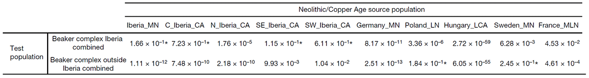
These and earlier results using Corded Ware as outgroup strongly suggest that early admixed Yamnaya Hungary samples (ca. 3100-2700 BC) will improve the fits for early East Bell Beaker groups (such as those of Southern Germany, Moravia, Silesia, or Northern Italy), especially when compared to a more northern R1a-M417-rich Proto-Corded Ware population from the Podolian-Volhynian Upland. On the other hand, later Bell Beaker samples outside of the core area will probably still need a fine-tuning with pre-BBC outgroups such as local neighbouring populations, including Steppe-related (Corded Ware) and/or EEF-related groups. Olalde et al. (2018) already tested some among the latter for all BBC groups:
Conclusion
The simplistic qpAdm assessment above is purely theoretical. I have explained elsewhere why formal stats are not the only relevant data when assessing admixture in general, and migration in particular. In fact, admixture models and proportions are quite possibly not even among the most relevant data for that. That’s why I introduced first the cultural and linguistic background, ancient phylogeography, and then showed the results of some simplistic (roughly age-equivalent) two-way qpAdm models. The latter cannot be understood without the former.
It is formally impossible to fully discard the thousand potential models whereby R1a-rich Corded Ware might have expanded as Bell Beakers from an eternally “yet-to-be-sampled” R1b-rich CWC group. Just as it is formally impossible to fully discard the thousand potential models whereby an eternally “yet-to-be-sampled” R1a-rich (Pre-)Yamnaya group might have expanded as the Proto-Corded Ware population, or the thousand potential models whereby an eternally “yet-to-be-sampled” R1b-rich EEF-like population might have expanded eastward as Proto-Beakers up to Hungary.
NOTE. For the latest model, you only need to select one low steppe population from France and a Corded Ware source rich in Steppe ancestry, and make your stepped qpAdm way eastwards up to Hungary, assuming ‘hidden’ populations, using dubious cultural attributions and questioning ancient phylogeography all the way to the steppes. The finding of good fits for Iberia CA (together with those for GAC) for Steppe-related groups in Wang et al. (2018) already showed that it’s possible. Another question entirely is why would someone try to show that (or an origin of BBC in CWC, for that matter) in 2020…
Luckily enough, data from Olalde et al. (2018) already hinted at the higher variability of “Steppe ancestry” precisely among (late) Hungary Bell Beakers with a likely direct origin in Moravia. Olalde et al. (2019) showed that Galaico-Lusitanians derive from a Germany BBC-like population, and Celtiberians from France BBC-like one (see here), and the recent finding of R1b-rich Italic and Palafitte-Terramare samples continuing low steppe Italy BBC-like peoples put an end to theories that involve an origin of North-West Indo-Europeans to the north of the Danube.
On the bright side, as the recent Preda-Bălănică, Frînculeasa, & Heyd (2020) state, no straightforward model can account for the complexity of this process in such a large area. The alternative visions – be it “top-to-down and broad-brush approach” as Kristiansen et al. (2017), or “bottom-up, detailed multidisciplinary regional” and continuist as Furholt (2019) – might still have some use to evaluate the main hypotheses for the different Bell Beaker groups, ranging between the three cornerstones: violence (=radical replacement), exchange (=heavy admixture), and neutrality (=resurgence events of local populations).
From a linguistic perspective, these regional interactions between Bell Beakers and late (Epi-)Corded Ware groups in Central and Northern Europe are precisely those which will help us determine the specific populations that better fit the known ancient contacts between early Indo-European and Uralic dialects in Europe, coupled with a proper dialectalization scheme and careful assessment of hydrotoponymic layers.
At least part of that obsessive effort in population genomics to continue simplistic and superficial archaeological and linguistic ideas of the past century will not go to waste.
Related
- Fully Steppe-like Proto-Corded Ware Late Trypillians
- “Steppe ancestry” step by step (2019): Mesolithic to Early Bronze Age Eurasia
- Bell Beakers and Mycenaeans from Yamnaya; Corded Ware from the forest steppe
- On the Ukraine Eneolithic outlier I6561 from Alexandria
- Yamnaya replaced Europeans, but admixed heavily as they spread to Asia
- East Bell Beakers, an in situ admixture of Yamna settlers and GAC-like groups in Hungary
- Trypillia and Greece Neolithic outliers: the smoking gun of Proto-Anatolian migrations?
- Corded Ware culture origins: The Final Frontier
- Volga Basin R1b-rich Proto-Indo-Europeans of (Pre-)Yamnaya ancestry
- Yamnaya ancestry: mapping the Proto-Indo-European expansions